1ª forma de resolução:

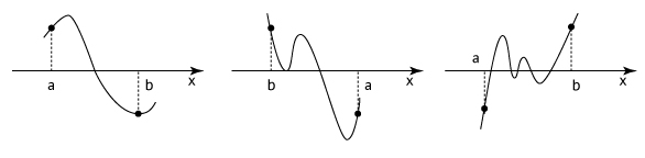
Para qualquer função polinomial  p, se p(a) e p(b) tiverem sinais contrários, então p tem pelo menos uma raiz real entre a e b. As figuras a seguir ilustram essa afirmação em diferentes casos através do gráfico de p:

 

No caso específico do polinômio , tem-se (valores escolhidos em função das alternativas):

Como P(1) e P(2) têm sinais contrários, pode-se concluir que P tem pelo menos uma raiz real r tal que 1 < r < 2.

Resposta: alternativa B

 

2ª forma de resolução:

As raízes de P(x) são dadas pela equação:

a qual pode ser reescrita como:

Resolver essa última equação equivale a encontrar as abscissas dos pontos de interseção dos gráficos dos polinômios . Esboçando-se ambos em um mesmo plano cartesiano, tem-se:

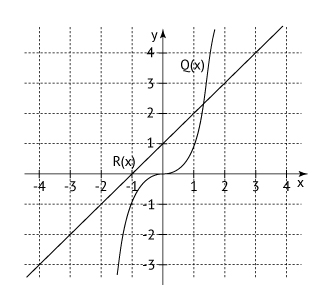
Pela figura, conclui-se que os gráficos se intersectam em apenas um ponto, de abscissa entre 1 e 2.

Resposta: alternativa B